0%

MATLAB 数字图像处理笔记

使用 MATLAB 图像处理工具箱做程序设计相对简单,本文通过几个可运行的小例子,梳理图像处理的常见技术:图像读写、颜色空间、直方图及均衡化、平滑滤波、边缘检测、二值化、降噪与形态学操作,帮助建立这方面的技能体系。原文写于 2018 年,首发于博客园,现迁移到本博客。

1 图像、视频文件读取

1
2
3
4
5
6
7
8
9
10
11
12
13
14
15
16
17
18
19
20
clear all; close all; clc;

% Read an image
A = imread('lena.jpg');

% Display the read image
figure, imshow(A);

% Print height, width and number of channels of the read image
height = size(A, 1);
width = size(A, 2);
number_of_channels = size(A, 3);

% Resize the image to 2x and display
B = imresize(A, 2.0);
figure, imshow(B);

% Rotate the image 逆时针旋转
C = imrotate(A, 90);
figure, imshow(C);

关键点:imread,figure(imshow),size 获取高度、宽度、图像通道数的参数,图像缩放,旋转。

1
2
3
4
5
6
7
8
9
10
11
12
clear all; close all; clc;

% Read an image
A = imread('lena.jpg');

% Translate the image
A_trans = imtranslate(A, [5 15]);

% Write the transformed image to disk
imwrite(A_trans, 'newlena.jpg');

figure, imshow(A_trans);

关键:imwrite 及其调用前做的工作。

1.1 视频读取(选看)

1
2
3
4
5
6
7
8
9
10
11
12
13
14
15
16
17
18
19
20
21
22
23
clear all; close all; clc;

% Initialize an object for reading video
videoObj = vision.VideoFileReader('video1.mp4', 'ImageColorSpace', 'RGB');
% Get video frame size and frame rate
S = info(videoObj);
width = S.VideoSize(1);
height = S.VideoSize(end);
frame_rate = S.VideoFrameRate;

% Get individual video frames
image_data = step(videoObj);

% Run the loop until all frames have been displayed
while ~isDone(videoObj)
% Display video frame one by one
imshow(image_data);

image_data = step(videoObj);
end

% Release the object for reading video
release(videoObj);

关键:step。其流程是 reader 读取生成对象,得到信息,逐帧显示。PS:视频教程中有另外一种实现。

2 图像格式

2.1 RGB、灰度图片

1
2
3
4
5
6
7
8
9
10
11
12
13
14
clear all; close all; clc;

% Read a RGB image
A = imread('lena.jpg');

% Verify number of channels
number_of_channels = size(A, 3)

% Convert RGB image to Grayscale
A_gray = rgb2gray(A);
number_of_channels2 = size(A_gray, 3)

figure, subplot(1, 2, 1), imshow(A), title('Input RGB image');
subplot(1, 2, 2), imshow(A_gray), title('Converted Grayscale image');

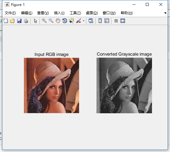
RGB 转灰度

关键:灰度图像颜色通道为 1,RGB 图像颜色通道数是 3,subplot 显示多个图像,便于查看。

2.2 RGB 与 HSV 通道

1
2
3
4
5
6
7
8
9
10
11
12
13
14
15
16
17
18
19
20
21
22
23
24
25
26
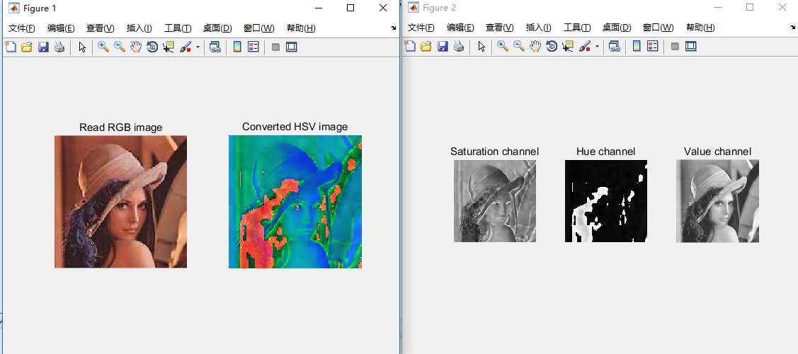
clear all; close all; clc;

% Read a RGB image
A = imread('lena.jpg');

% Extract individual R, G & B channels from RGB image
R = A(:, :, 1);
G = A(:, :, 2);
B = A(:, :, 3);

% Convert RGB image to HSV color space
A_hsv = rgb2hsv(A);

% Extract individual H, S & V channels from HSV image
H = A_hsv(:, :, 1);
S = A_hsv(:, :, 2);
V = A_hsv(:, :, 3);

% Display the read RGB image and HSV converted image
figure, subplot(1, 2, 1), imshow(A), title('Read RGB image');
subplot(1, 2, 2), imshow(A_hsv), title('Converted HSV image');

% Displaying individual image channels.
figure, subplot(1, 3, 1), imshow(S), title('Saturation channel');
subplot(1, 3, 2), imshow(H), title('Hue channel');
subplot(1, 3, 3), imshow(V), title('Value channel');

RGB 与 HSV 通道

关键:R、G、B、H、S、V 都是提取空间域(矩阵表示)的信息,为图片大小。RGB、HSV 格式都是 3 个颜色通道,前者 uint8,后者 double 格式。PS:HSV 有用的是 V(当前)。

3 直方图

直方图以前都是空间域上对像素操作,直方图则是借助频率来获取图像的统计信息:imhist。

1
2
3
4
5
6
7
8
9
10
11
12
13
14
clear all; close all; clc;

% Read an image
A = imread('lena.jpg');
B = imread('lena.jpg');

% Convert the read image to single-channel
A = rgb2gray(A);

% Plot and display the histogram if A is a single channel image with
% default number of bins
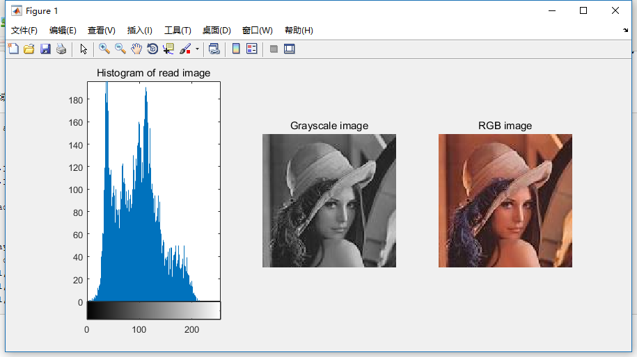
figure, subplot(1,3,1), imhist(A), title('Histogram of read image');
subplot(1,3,2), imshow(A), title('Grayscale image');
subplot(1,3,3), imshow(B), title('RGB image');

灰度图直方图

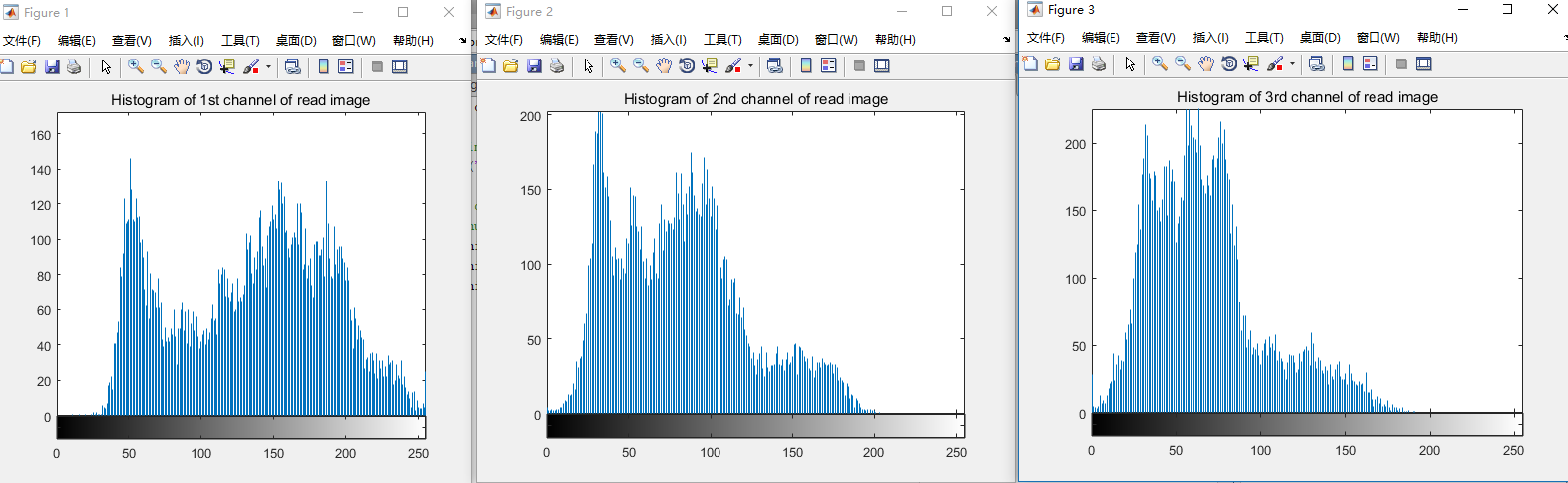
直方图:左边暗,右边亮,表示不同亮度出现的频率。注意直方图应该表示一个颜色通道的统计信息,不要把 RGB、HSV 等格式图片多个通道的格式混合起来,这样是得不到可分析的信息的。RGB 直方图生成方式如下:

1
2
3
4
5
6
7
8
9
10
clear all; close all; clc;

% Read an image
A = imread('lena.jpg');

% Plot and display the histogram if A is a 3 channel image with
% default number of bins
figure, imhist(A(:, :, 1)), title('Histogram of 1st channel of read image');
figure, imhist(A(:, :, 2)), title('Histogram of 2nd channel of read image');
figure, imhist(A(:, :, 3)), title('Histogram of 3rd channel of read image');

RGB 各通道直方图

4 直方图均衡化

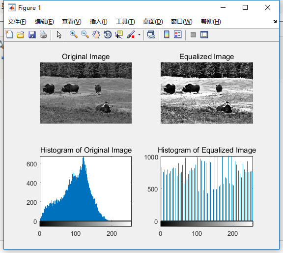
亮度分布集中在左边,图片太暗;集中在右边,图片太亮。直方图均衡化就是让图像的不同像素点亮度均匀化,对灰度图片和其他格式图片有不同的做法。

1
2
3
4
5
6
7
8
9
10
11
12
13
14
15
16
17
clear all; close all; clc;

% Read an image
A = imread('test1.jpg');

% Convert the image to single channel image
A = rgb2gray(A);

% Equalize the histogram of read single channel image
A_histeq = histeq(A);

% Display original and equalized images side by side with their respective
% histogram plots
figure, subplot(2, 2, 1), imshow(A), title('Original Image');
subplot(2, 2, 2), imshow(A_histeq), title('Equalized Image');
subplot(2, 2, 3), imhist(A), title('Histogram of Original Image');
subplot(2, 2, 4), imhist(A_histeq), title('Histogram of Equalized Image');

灰度图直方图均衡化

关键:imhist,histeq。

1
2
3
4
5
6
7
8
9
10
11
12
13
14
15
16
17
18
clear all; close all; clc;

% Read a RGB image
A = imread('test1.jpg');

% Convert the RGB image into HSV image
A_hsv = rgb2hsv(A);

% Perform histogram equalization of V-channel in HSV image which is the 3rd
% channel
A_hsv(:, :, 3) = histeq(A_hsv(:, :, 3));

% Convert back equalized HSV image into RGB image
A_histeq = hsv2rgb(A_hsv);

% Display original and equalized RGB images side by side
figure, subplot(1, 2, 1), imshow(A), title('Original RGB image');
subplot(1, 2, 2), imshow(A_histeq), title('Equalized RGB image');

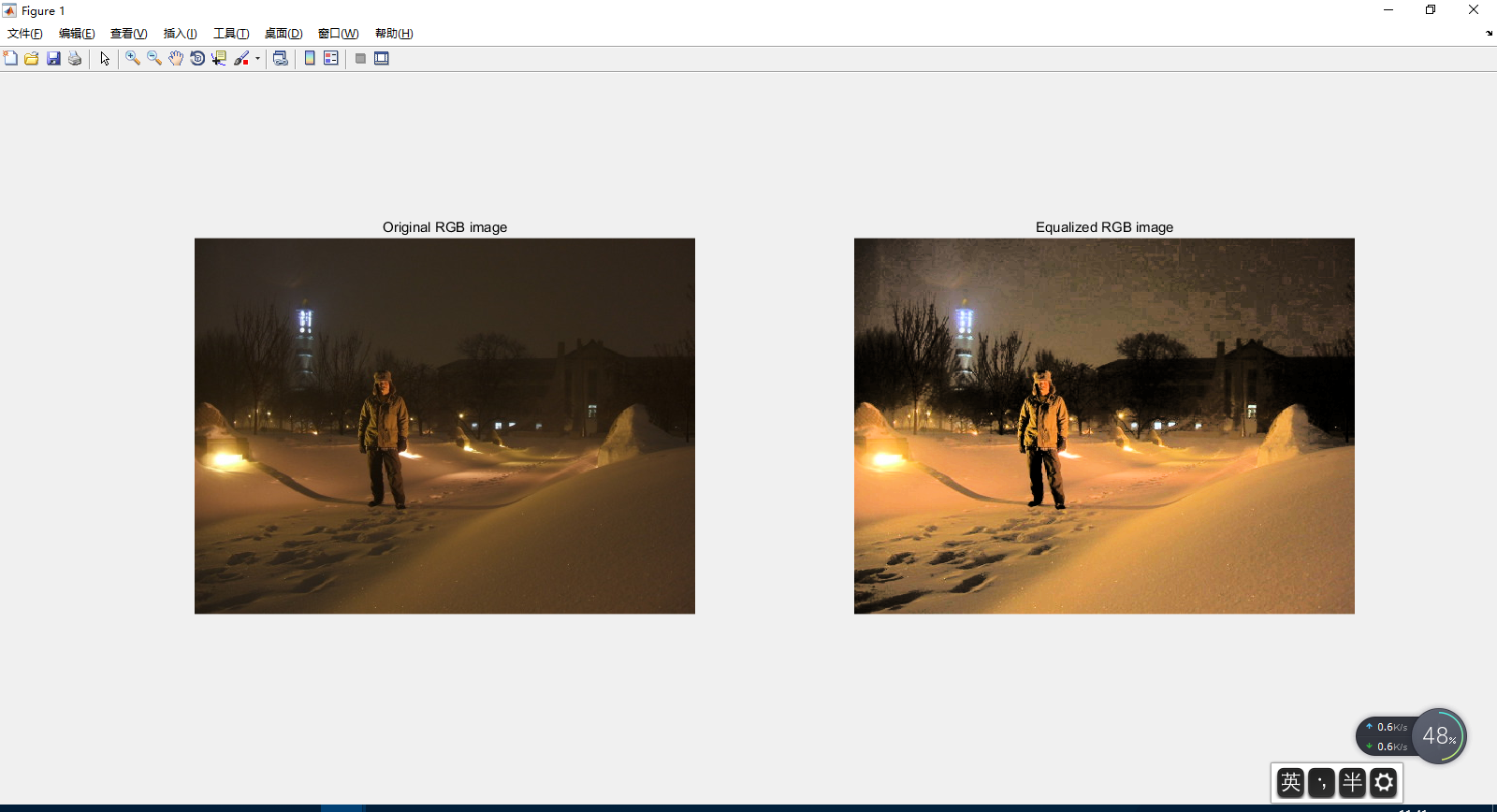
RGB 直方图均衡化

关键:histeq(A(:, :, 3)),A 是 HSV 格式。流程:RGB 图片转化为 HSV 图片,然后对 HSV 图片的 V 通道进行均衡化,均衡化后重新转化为 RGB 图片。

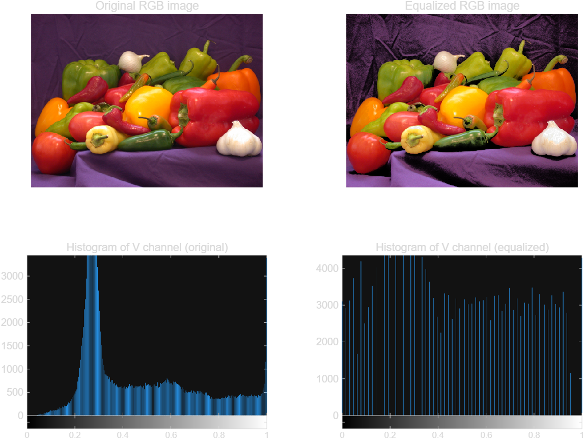
下面这张图是用 MATLAB 自带的 peppers.png 重做的演示(原图已失效):左上是原图,右上是均衡化后的结果,下面是 V 通道均衡前后的直方图对比,可以看到均衡化后亮度分布被拉开了。

V 通道均衡化前后对比

5 图像平滑化(image smoothing)

释义:消除、弱化、压缩图像的噪声、边缘、细节、突变。可以在空间域(滤波)和频域上进行。关键函数:fspecial、imfilter。

空间域:生成一个任意大小的矩阵,用该矩阵对图像某个像素及其周围像素进行集体操作后代替原像素。根据将像素值设置为不同的值类型,可以分为:最小化、最大化、均值、加权均值操作。

5.1 空间滤波示例

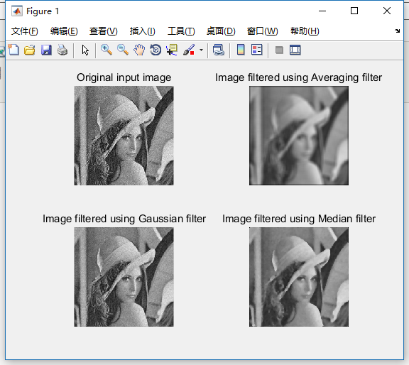
流程:生成灰度图像,生成滤波器,应用滤波,执行滤波操作。PS:中值滤波过程不一样。

1
2
3
4
5
6
7
8
9
10
11
12
13
14
15
16
17
18
19
20
21
22
23
24
25
26
27
28
clear all; close all; clc;

% Read an input image
A = imread('test1.jpg');

% Conversion to single channel image
A = rgb2gray(A);

% Generate Average filter
average_h = fspecial('average', [9 9]);

% Generate Gaussian filter
gaussian_h = fspecial('gaussian', [13 13]);

% Filter input image using average filter
B_average = imfilter(A, average_h);

% Filter input image using Gaussian filter
B_gaussian = imfilter(A, gaussian_h);

% Filter input image using median filter
B_median = medfilt2(A, [5 5]);

% Display input and filtered images side by side
figure, subplot(2, 2, 1), imshow(A), title('Original input image');
subplot(2, 2, 2), imshow(B_average), title('Image filtered using Averaging filter');
subplot(2, 2, 3), imshow(B_gaussian), title('Image filtered using Gaussian filter');
subplot(2, 2, 4), imshow(B_median), title('Image filtered using Median filter');

四种平滑滤波对比

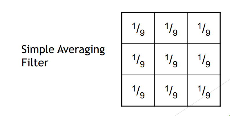
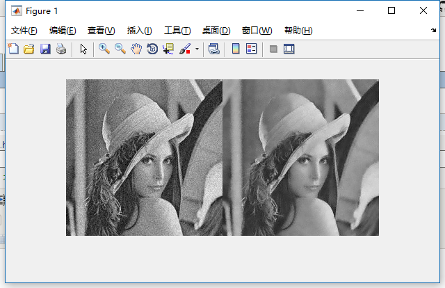
均值滤波是最简单的空间滤波,特点:1、非加权;2、适用于去噪声,但会使图片模糊;3、突出总体细节。

均值滤波

5.2 加权平滑滤波器

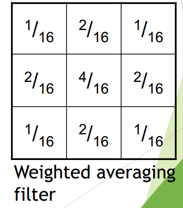
pixel 有不同权值的滤波器,特点:越靠近中心的像素越重要;与非权值的滤波操作(均值滤波)相比,更好的模糊化。滤波器构造如下图所示。

加权滤波器构造

加权滤波器

补充一个导向滤波的例子,这么做的目的是保留图像的边缘。

1
2
3
4
5
6
7
8
9
10
clear all; close all; clc;

% Read an image
A = imread('test1.jpg');

% Filter the image using guided filter
A_guided_filtered = imguidedfilter(A);

% Display original and processed image side-by-side
imshowpair(A, A_guided_filtered, 'montage');

导向滤波

6 边缘检测

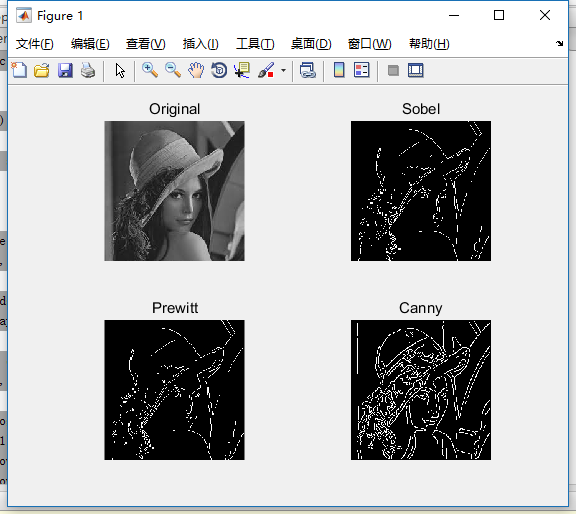
边缘是重要的图像强度局部变化像素点的集合。边缘方向:垂直于图像强度最大强度变化的方向。

思路:空间域上对 x、y 求导,大于特定的值就是边缘,不同的算子生成方式有不同的近似求导方案。

1
2
3
4
5
6
7
8
9
10
11
12
13
14
15
16
17
18
19
20
21
22
23
clear all; close all; clc;

% Read an image
A = imread('test1.jpg');

% Convert the image to single-channel intensity image if the read image
% is RGB (3-channel)
A_gray = rgb2gray(A);

% Method for Sobel edge detection
BW_sobel = edge(A_gray, 'sobel');

% Method for Prewitt edge detection
BW_prewitt = edge(A_gray, 'prewitt');

% Method of Canny edge detection
BW_canny = edge(A_gray, 'canny');

% Display the images together
figure, subplot(2, 2, 1), imshow(A_gray), title('Original');
subplot(2, 2, 2), imshow(BW_sobel), title('Sobel');
subplot(2, 2, 3), imshow(BW_prewitt), title('Prewitt');
subplot(2, 2, 4), imshow(BW_canny), title('Canny');

Sobel、Prewitt、Canny 边缘检测对比

7 二值图像(im2bw)

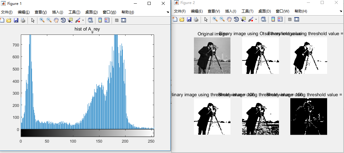
图像只有两个值 0、1。根据直方图左边暗、右边亮,左边取 0(黑),右边取 1(白)。二值图像是根据直方图,大于某个值则设置为 1(白色),二值图像生成的关键就是这个阈值的选择,否则二值图像生成的背景、人物、物体会杂糅在一起,没有办法继续处理。

流程:灰度 → double → im2bw,第 2 个参数要 ∈ [0, 1],阈值除以 255 带入。PS:Otsu 算法已经集成在 MATLAB 工具箱中了。

1
2
3
4
5
6
7
8
9
10
11
12
13
14
15
16
17
18
19
20
21
22
23
24
25
26
27
28
29
30
31
clear all; close all; clc;

% Read an input image
A = imread('test1.jpg');

% Convert the image to single-channel grayscale image
A_gray = rgb2gray(A);

figure, imhist(A_gray), title('hist of A_grey');

% Convert image to double i.e., [0,1]
A_gray = im2double(A_gray);

% Generate threhold value using Otsu's algorithm
otsu_level = graythresh(A_gray);

% Threshold image using Otsu's threshold and manually defined
% threshold values
B_otsu_thresh = im2bw(A_gray, otsu_level);
B_thresh_50 = im2bw(A_gray, 50/255);
B_thresh_100 = im2bw(A_gray, 100/255);
B_thresh_150 = im2bw(A_gray, 150/255);
B_thresh_200 = im2bw(A_gray, 200/255);

% Display original and thresholded binary images side-by-side
figure, subplot(2, 3, 1), imshow(A_gray), title('Original image');
subplot(2, 3, 2), imshow(B_otsu_thresh), title('Binary image using Otsu threshold value');
subplot(2, 3, 3), imshow(B_thresh_50), title('Binary image using threshold value = 50');
subplot(2, 3, 4), imshow(B_thresh_100), title('Binary image using threshold value = 100');
subplot(2, 3, 5), imshow(B_thresh_150), title('Binary image using threshold value = 150');
subplot(2, 3, 6), imshow(B_thresh_200), title('Binary image using threshold value = 200');

不同阈值的二值化对比

8 图像降噪(fspecial、imfilter)

噪声来源于图像采集及转化、传输过程。

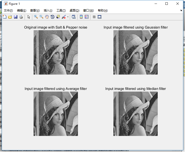
噪声分类:高斯噪声,正态分布;椒盐噪声,一定概率分布的黑白像素点;冲击噪声,随机白点。

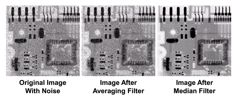
降噪手段:最简单的是均值滤波,但是会模糊整个图片;中值滤波适用于椒盐噪声。

周期性的噪声多来自于电子电磁干扰,噪声在图像中的分布具有规律性(周期性),傅里叶域的频域技术在消除周期性噪声时是最有效的。带阻滤波适合移除图片噪声及移除特定范围的频率。

1
2
3
4
5
6
7
8
9
10
11
12
13
14
15
16
17
18
19
20
21
22
23
24
clear all; close all; clc;

% Read an input image
A = imread('test1.jpg');

% Generate Gaussian and Average filters
h_gaussian = fspecial('gaussian');
h_average = fspecial('average');

% Filter input image using generated Gaussian and Average filters
B_gaussian = imfilter(A, h_gaussian);
B_average = imfilter(A, h_average);

% Filter input image using Median filter
% Median filtering function takes as input grayscale image
A_gray = rgb2gray(A);
B_median = medfilt2(A_gray);

% Display original and filtered images side-by-side for comparing the
% result of image de-noising
figure, subplot(2, 2, 1), imshow(A), title('Original image with Salt & Pepper noise');
subplot(2, 2, 2), imshow(B_gaussian), title('Input image filtered using Gaussian filter');
subplot(2, 2, 3), imshow(B_average), title('Input image filtered using Average filter');
subplot(2, 2, 4), imshow(B_median), title('Input image filtered using Median filter');

三种降噪滤波对比

9 形态学

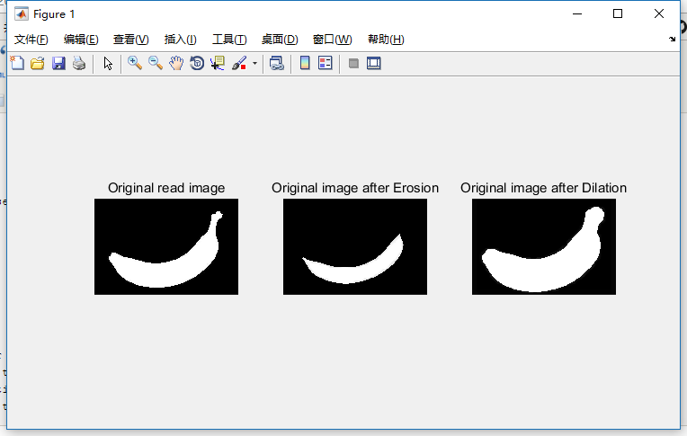
Erosion 腐蚀(imerode):分离相连物体,去毛刺,让物体变小;Dilation 膨胀(imdilate):拼接物体,填表面小坑,物体变大。

1
2
3
4
5
6
7
8
9
10
11
12
13
14
15
16
17
18
19
20
21
close all; clear all; clc;

% Read an input image
A = imread('binaryImg1.jpg');

% Convert to single channel
A = rgb2gray(A);

% Generate structuring element for use
se = strel('disk', 15);

% Perform image erosion
B_eroded = imerode(A, se);

% Perform image dilation
B_dilated = imdilate(A, se);

% Display the images side-by-side for comparison
figure, subplot(1, 3, 1), imshow(A), title('Original read image');
subplot(1, 3, 2), imshow(B_eroded), title('Original image after Erosion');
subplot(1, 3, 3), imshow(B_dilated), title('Original image after Dilation');

腐蚀与膨胀

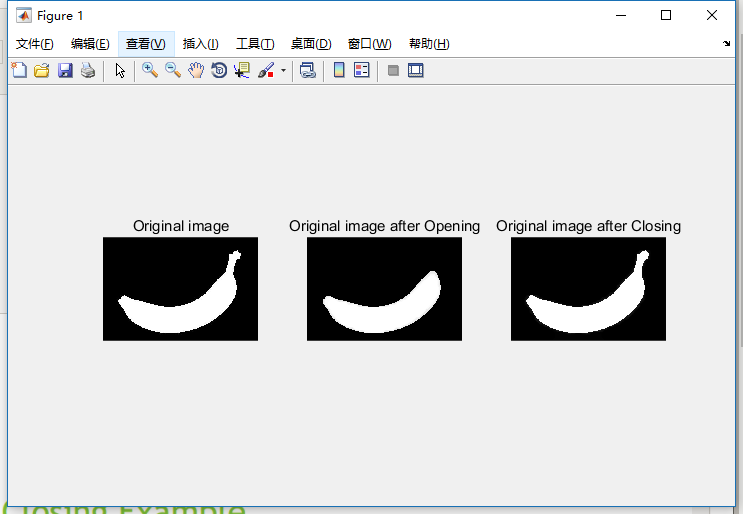
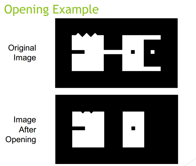
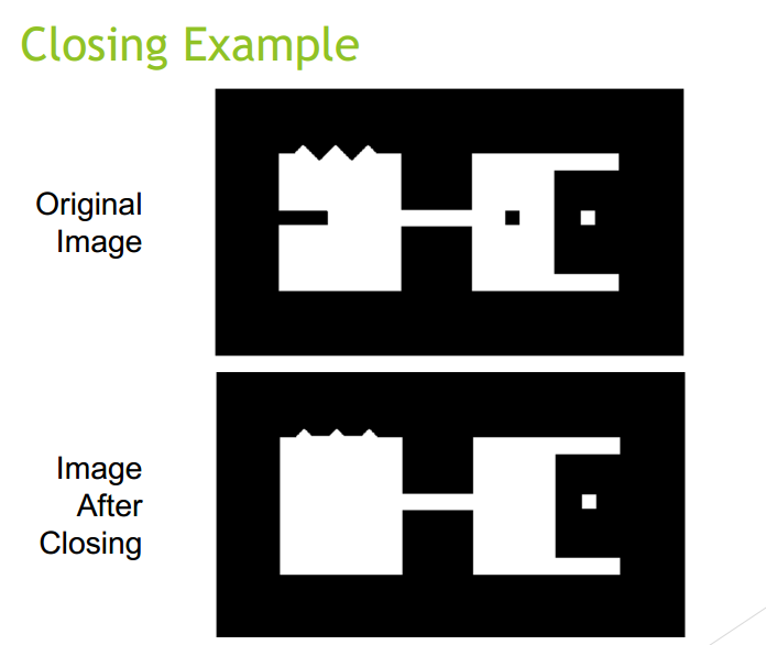
开运算:先腐蚀再膨胀,分离物体、去毛刺、去小点(物体点)、去小部件,表面坑变小。
闭运算:先膨胀再腐蚀,表面坑被填,内部背景点消失,毛刺不变。

1
2
3
4
5
6
7
8
9
10
11
12
13
14
15
16
17
18
19
20
21
clear all; close all; clc;

% Read an input image
A = imread('binaryImg1.jpg');

% Convert read image to single channel image
A = rgb2gray(A);

% Generate structuring element for processing
se = strel('disk', 15);

% Perform image opening operation
B_open = imopen(A, se);

% Perform image closing operation
B_close = imclose(A, se);

% Display original and processed images
figure, subplot(1, 3, 1), imshow(A), title('Original image');
subplot(1, 3, 2), imshow(B_open), title('Original image after Opening');
subplot(1, 3, 3), imshow(B_close), title('Original image after Closing');

开运算与闭运算

开闭运算效果

形态学示意

形态学示意

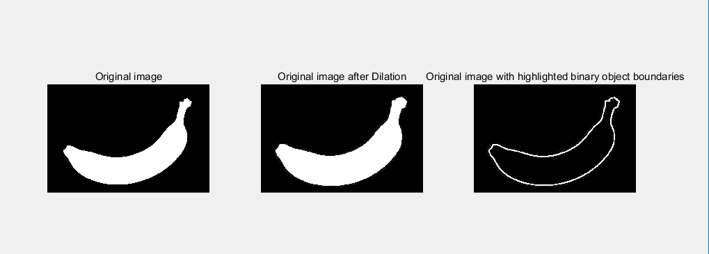
9.1 利用膨胀得到物体边缘

1
2
3
4
5
6
7
8
9
10
11
12
13
14
15
16
17
18
19
20
21
22
23
clear all; close all; clc;

% Read an input image
A = imread('binaryImg1.jpg');

% Convert the read image to single channel image
A = rgb2gray(A);

% Generate structuring element for use
se = strel('disk', 5);

% Perform image dilation
% To get the object boundary, subtract the original image from the dilated
% version of the orginal image
B_dilated = imdilate(A, se);

% Subtract the original image from dilated image
B_boundary = B_dilated - A;

% Display images side by side
figure, subplot(1, 3, 1), imshow(A), title('Original image');
subplot(1, 3, 2), imshow(B_dilated), title('Original image after Dilation');
subplot(1, 3, 3), imshow(B_boundary), title('Original image with highlighted binary object boundaries');
膨胀法提取边缘

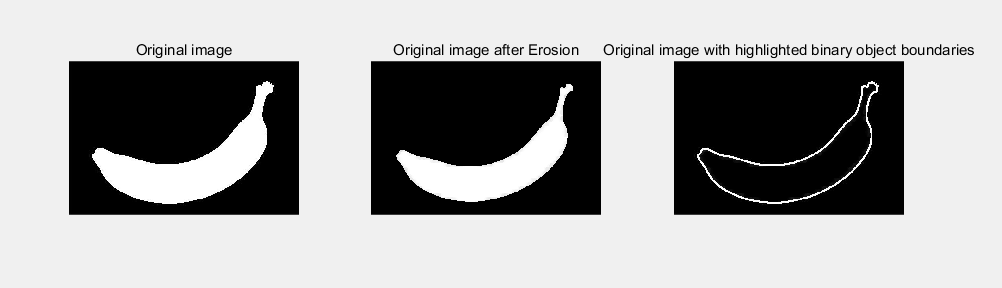
9.2 利用腐蚀得到物体边缘

1
2
3
4
5
6
7
8
9
10
11
12
13
14
15
16
17
18
19
20
21
clear all; close all; clc;

% Read an input image
A = imread('binaryImg1.jpg');

% Convert the read image to single channel image
A = rgb2gray(A);

% Generate structuring element for use
se = strel('disk', 5);

% Perform image erosion
B_eroded = imerode(A, se);

% Subtract the eroded image from original image
B_boundary = A - B_eroded;

% Display images side by side
figure, subplot(1, 3, 1), imshow(A), title('Original image');
subplot(1, 3, 2), imshow(B_eroded), title('Original image after Erosion');
subplot(1, 3, 3), imshow(B_boundary), title('Original image with highlighted binary object boundaries');
腐蚀法提取边缘